Behind the scenes | automatic quadrat detection
The idea of putting together an automatic quadrat detection algorithm was not in photoQuad's initial design plans. After some numerous manual detection efforts however, it was becoming obvious that the purely manual approach was a bottleneck in the overall image preparation time, and a semi-automatic tool would be handy. So, how do you build such a tool and how do you make it work in different images?
The answer is that you need to take advantage of some quadrat characteristics that are consistent across images. Here's our best guess:
the quadrat frame is generally the brightest object in the image and has a relatively uniform color
if somehow isolated, the quadrat's effective sampling area (the inner portion of the quadrat) is the largest contiguous object in the image
With these observations in hand, a solution could be a series of image processing tricks such as binary conversion, image erosion, intensity thresholding, identification of connected components, filtering of connected objects based on their size, and boundary detection of the largest object.
A step by step overview is described below. It's not the smartest method possible, but it works, it's fast, and is fully automated.
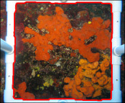
Step 1
A typical photoquadrat image.
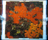
Step 2 | convert to grayscale
The original three-channel RGB image is converted to a one-channel grayscale image. This grayscale image actually contains pixel intensities ranging from the minimum value 0 (=black) to the maximum value 1 (=white); grays fall in between.
Nothing clever happens here, it's an intermediate step.
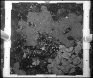
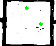
Step 3 | erode image (optional)
Erosion is a morphological operation that removes pixels on bright object boundaries (it shrinks objects), using structuring elements. To understand what a structuring element is, think of viewing portions of the image through a viewfinder: a custom-shaped element (e.g. a disk) slides over the image, reducing the brightness, therefore the size, of bright objects by assigning the neighborhood minimum to all pixels that are below the sliding element.
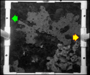
Compare the quadrat frame on the right with the image in Step 2. The quadrat is thinner or "eroded" (green arrow), and bright object boundaries are more clear-cut (yellow arrow).
Step 4 | inverse binary and intensity thresholding
A binary image has only two possible values for each pixel: either 0 (=black) or 1 (=white). Using the image from Step 3 as the source, pixels that are brighter than a threshold become white, the rest become black. Of course, the bright quadrat frame will turn out to be the white object here. We need the inverse, so we invert it.
Note that small blobs from initially bright image regions will always remain in the quadrat's active area (green arrows).
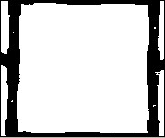
Step 5 | flood-fill
The flood-fill operation removes holes (i.e. black pixels) from the binary image, by "flooding" white regions. This is done in a controlled manner, so that only blobs from Step 4 are removed. Over-flooding will make the quadrat frame dissapear also, which is not very useful.
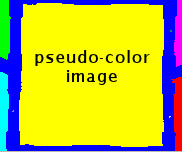
Step 6 | size matters
If we were to detect the connected components in the image from Step 5 and color them accordingly, the result would be something like the thumbnail on the right. By construction, the quadrat's active area (the yellow object) is bound to be the biggest object no matter what. So, we keep only the biggest object, and set all other pixels to zero (black).
Step 7 | trace boundary | image opening (optional)
For most photoquadrat cases, the process is over. The boundary of the white object is traced, converted into ordinary X,Y polygon coordinates, and superimposed on the original image.
If the boundary comes out too edgy or does not close properly (think of having an original image with a finger or seaweed ontop of the quadrat frame), an additional "image opening" process can smooth the result and correct discontinuities.

Step 8 | final image | system registration
From the user's perspective, the quadrat's inner boundary is just a polygon that is superimposed on the image, and that's how things should be.
System-wise however, the quadrat boundary is assinged to a distinct plotting layer, quadrat right-click functions are registered, the boundary is calibrated (if image calibration data exist), and photoQuad gathers "real-time" information about image regions or analysis objects that fall inside and outside the quadrat, so that analysis descriptors can be automatically updated. The good thing is that all of this happens in the background.